Darknet-Yolov3 移植过程
Darknet-Yolov3移植Cambricon-Caffe教程
前言
本教程面向使用寒武纪平台进行深度学习推理任务的开发者。针对当前主流检测网络darknet-yolov3,进行寒武纪平台的移植。开发者对照移植过程,能够利用寒武纪智能处理器设备完成多种场景的目标检测任务。
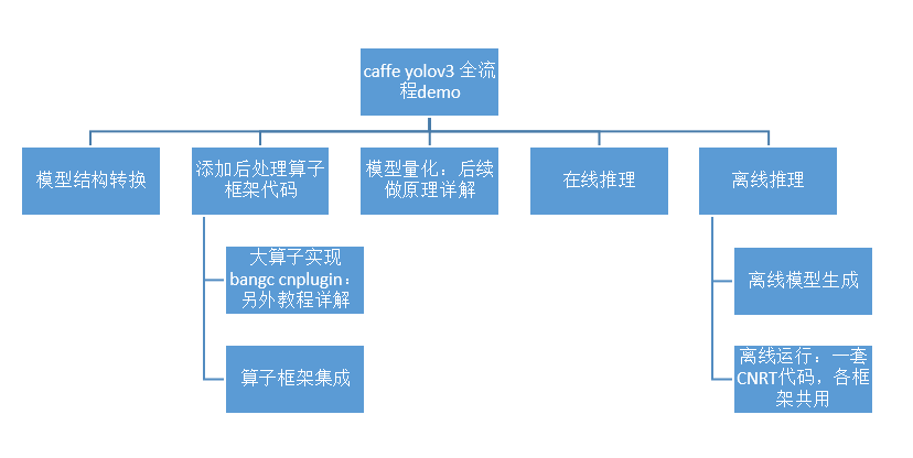
整个移植过程分为模型结构转换、添加后处理算子Caffe框架代码、模型量化、在线推理和离线推理共五个步骤,整个流程图如下:
本实验的相关代码和脚本运行步骤请见:https://github.com/CambriconECO/Caffe_Yolov3_Inference
本实验代码基于 Neuware 1.6.1 与 Python 2.7 环境。
一、模型结构转换
注意:Model Zoo中的官方网络大部分可以跳过这一步,直接进入量化步骤。由于yolov3没有官方的Caffe网络模型,所以我们要进行一定的修改才能进入量化步骤。修改的内容主要是在原有的backbone网络的后面添加后处理大算子从而实现完成的检测过程。
1. Yolov3没有官方的Caffe网络模型,如果要在Cambricon Caffe上使用yolov3网络,需要将原有cfg文件转换成yolov3.prototxt文件,将yolov3.weights转换成yolov3.caffemodel。这部分转换可以使用Cambricon Caffe自带工具实现,示例如下:
python darknet2caffe-yoloV23.py 3 yolov3.cfg yolov3.weights yolov3.prototxt yolov3.caffemodel
参数说明:
3 # 针对不同yolov网络的选项 2代表yolov2 3代表yolov3
yolov3.cfg # yolov3配置文件路径
yolov3.weights # yolov3权重路径
yolov3.prototxt # 要生成的.prototxt名
yolov3.caffemodel # 要生成的.caffemodel名
使用这个工具会将cfg文件中定义的网络转换成不带后处理大算子的网络部分结构。
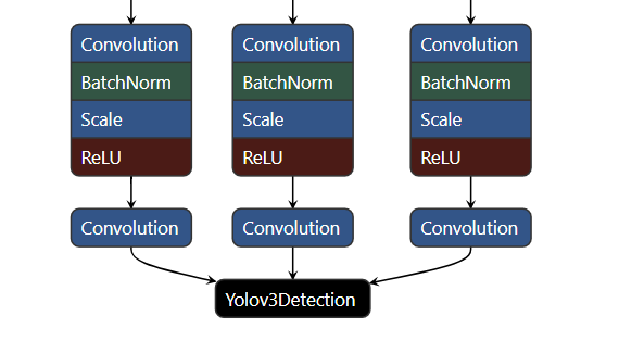
2. 另外对于原始Yolov3网络的后处理部分的逻辑,Cambricon Caffe推荐使用一个大的BANGC算子完成后处理的计算(含nms),进一步提高运行效率。所以这部分需要对原生的Caffe网络进行修改,向prototxt中添加Yolov3Detection算子节点,即在末尾添加后处理层,输入为原生网络的三个最终输出:
layer {
name: "yolo-layer"
type: "Yolov3Detection"
bottom: "layer82-conv"
bottom: "layer94-conv"
bottom: "layer106-conv"
top: "yolo_1"
yolov3_param {
num_box: 1024
confidence_threshold: 0.5
nms_threshold: 0.45
im_w: 416
im_h: 416
biases:[116,90,156,198,373,326,30,61,62,45,59,119,10,13,16,30,33,23]
}
}
最终修改后的效果如图所示:
二、Caffe框架添加后处理算子
在第一步中我们使用了BANGC编写的Yolov3Detection算子替换掉了原始的后处理逻辑,为了保证能够正确调用到这个算子,我们需要将该Yolov3Detection算子集成到框架中,共分成两步:以pluginop的形式封装,集成到CNPlugin中,然后将CNPlugin算子集成到Cambricon Caffe。该算子的实现与集成到CNPlugin会在另一个教程中详细介绍,在这里只介绍将该算子集成到Cambricon Caffe这一步骤。
操作步骤:
1. 在<caffe>/src/caffe/proto/caffe.proto中添加层的参数和计算引擎。这使得Caffe在创建层时能根据特定的引擎选择构造的对象。
message Yolov3DetectionParameter {
// Yolo detection output layer
optional int32 num_classes = 1 [default = 80];
optional int32 num_box = 2 [default = 1024];
optional float confidence_threshold = 3 [default = 0.5];
optional float nms_threshold = 4 [default = 0.45];
optional int32 anchor_num = 5 [default = 3];
repeated float biases = 6;
optional int32 im_w = 7 [default = 416];
optional int32 im_h = 8 [default = 416];
enum Engine {
DEFAULT = 0;
CAFFE = 1;
MLU = 2;
} // 可对照到第④步进行查看
optional Engine engine = 9 [default = DEFAULT];
}
2. 添加头文件<caffe>/include/caffe/layers/mlu_yolov3_detection_layer.hpp。头文件的具体代码应当包含在#ifdef USE_MLU⋯#endif和namespacecaffe中。每个层都应当显式地添加下面的这些函数声明。这些函数的被调用策略请参考<caffe>/include/caffe/layer.hpp。
template <typename Dtype>
class MLUYolov3DetectionLayer : public Yolov3DetectionLayer<Dtype> {
public:
explicit MLUYolov3DetectionLayer(const LayerParameter& param)
: Yolov3DetectionLayer<Dtype>(param), yolo_op_ptr_(nullptr),
yolov3_ptr_param_(nullptr) {}
virtual void LayerSetUp(const vector<Blob<Dtype>*>& bottom,
const vector<Blob<Dtype>*>& top);
virtual void Reshape_tensor(const vector<Blob<Dtype>*>& bottom,
const vector<Blob<Dtype>*>& top);
// 在线融合模式要添加下面两个接口
// 1)融合操作。融合模式需要将本层的算子融合进接口传来的融合器中,融合的步骤应当和算子的创建(或在线逐层模式Forward中对各个算子的Forward计算)拥有类似的判断。
virtual void fuse(MFusion<Dtype>* fuser);
// 2)复写mfus_supported()。将本层标记为支持融合模式。
virtual inline bool mfus_supported() { return true; }
virtual ~MLUYolov3DetectionLayer();
protected:
virtual void MLUDestroyOp();
virtual void MLUCreateOpBindData(const vector<Blob<Dtype>*>& bottom,
const vector<Blob<Dtype>*>& top);
virtual void MLUCompileOp();
virtual void Forward_mlu(const vector<Blob<Dtype>*>& bottom,
const vector<Blob<Dtype>*>& top);
shared_ptr<Blob<Dtype>> buffer_blob_; // buffer gdram for multicore
shared_ptr<Blob<Dtype>> fake_input_blob0_; // fake input
cnmlBaseOp_t yolo_op_ptr_;
cnmlPluginYolov3DetectionOutputOpParam_t yolov3_ptr_param_;
};
3. 添加源文件<caffe>/src/caffe/layers/mlu_yolov3_detection_layer.cpp。和头文件一样,源文件的位置也在#ifdef USE_MLU⋯#endif和namespacecaffe中间。源文件对各个接口的具体实现方法各有不同,具体可打开源文件查看。
4. 在<caffe>/src/caffe/layer_factory.cpp中增加层的注册功能。上述步骤中定义并增加了新的层,在使用之前还需要修改Caffe创建层的逻辑。
// Get yolov3 Layer according to engine
template <typename Dtype>
shared_ptr<Layer<Dtype>> GetYolov3DetectionLayer(const LayerParameter& param) {
Engine engine = param.engine();
if (engine == Engine::DEFAULT) {
engine = Engine::CAFFE;
#ifdef USE_MLU
engine = Engine::MLU;
#endif
}
if (engine == Engine::CAFFE) {
return shared_ptr<Layer<Dtype>>(new Yolov3DetectionLayer<Dtype>(param));
#ifdef USE_MLU
} else if (engine == Engine::MLU) {
if (Caffe::mode() == Caffe::MLU || Caffe::mode() == Caffe::MFUS)
return shared_ptr<Layer<Dtype>>(new MLUYolov3DetectionLayer<Dtype>(param));
else
return shared_ptr<Layer<Dtype>>(new MLUYolov3DetectionLayer<Dtype>(param));
#endif
} else {
LOG(FATAL) << "Layer " << param.name() << "has unknown engine.";
throw;
}
}
REGISTER_LAYER_CREATOR(Yolov3Detection, GetYolov3DetectionLayer);
三、模型量化
为什么要量化:量化是将float32的模型转换为int8/int16的模型,可以保证计算精度在目标误差范围内的情况下,显著减少模型占用的存储空间和处理带宽,已提高模型推理性能。如int8模型是指将数值以有符号8位整型数据保存,并提供int8定点数的指数position和缩放因子scale,因此int8模型中每个8位整数i表示的实际值为:value=( i*2^position ) / scale。进行在线推理和生成离线模型时仅支持输入量化后的模型。
操作步骤:
1. 对上一步生成的protoxt进行量化时,首先要配置ini文件,打开./quantize/convert_quantized.ini,修改配置如下:
[model]
;blow two are lists, depending on framework
original_models_path = ./yolov3.prototxt
save_model_path = ./yolov3_int8.prototxt
;input_nodes = input_node_1
;output_nodes = output_node_1, output_node_2
[data]
;only one should be set for below two
;images_db_path = /path/to/caffe_data_models/data/ilsvrc12_val_lmdb/
images_list_path = ./images.lst
used_images_num = 1
[weights]
original_weights_path = ./yolov3.caffemodel
[preprocess]
;mean value order should be the same as filter channel order
mean = 0, 0, 0
;support single std and channel std, channel order should be the same as filter channel order
;std=1/255
std = 0.00392157
scale = 416,416
crop = 416,416
[config]
quantize_op_list = Conv, FC, LRN
use_firstconv = 1
;customer configuration
[custom]
use_custom_preprocess = 0
;only support ARGB, ABGR, BGRA, RGBA
;input_format = ARGB
;only support BGR, RGB
;filter_format = BGR
参数说明:
*originl_models_path:第一步修改后的prototxt路径,即待量化的原始网络;
*save_model_path:即将生成的int8的prototxt路径,即量化后的网络;
*images_list_path:图片列表文件路径,images.lst存储了量化时需要的图片路径,量化时使用一张图片即可;
*used_images_num:迭代的次数,网络的batch为1,used_images_num为8,共迭代8次,读取8 张图。网络的batch为4,used_images_num为8,共迭代8次,读取32张图;
*original_weights_path:待量化网络的caffemodel路径;
*mean:均值;
*std:缩小倍数;
*scale:输入图像的高度和宽度;
*crop:裁剪的高度和宽度;
*use_firstconv:是否使用到firstconv。 1代表使用,0代表不使用。
2. 修改完成后,就可以使用Cambricon Caffe自带工具进行量化,示例如下:
./generate_quantized_pt --ini_file convert_quantized.ini
注意:如果使用量化后的模型进行推理时,发现推理结果不对,那么很有可能是量化时的mean和std参数设置的不对。量化时的数据预处理参数和一般情况下推理的数据预处理参数要保持一致。
四、在线推理
在线推理分为在线逐层推理和在线融合推理:
1. 融合模式:被融合的多个层作为单独的运算(单个 Kernel)在 MLU 上运⾏。根据⽹络中的层是否可以被融合,⽹络被拆分为若⼲个⼦⽹络。 MLU 与 CPU 间的数据拷⻉只在各个⼦⽹络之间发⽣。⼀般认为在线融合模式⽐在线逐层模式运⾏速度更快。
2. 逐层模式:逐层模式中,每层的操作都作为单独的运算(单个 Kernel)在 MLU 上运⾏,⽤⼾可以将每层结果导出到 CPU 上,⽅便⽤⼾进⾏调试。
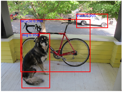
执行在线逐层推理,示例如下:
python detect.py yolov3_int8.prototxt yolov3.caffemodel
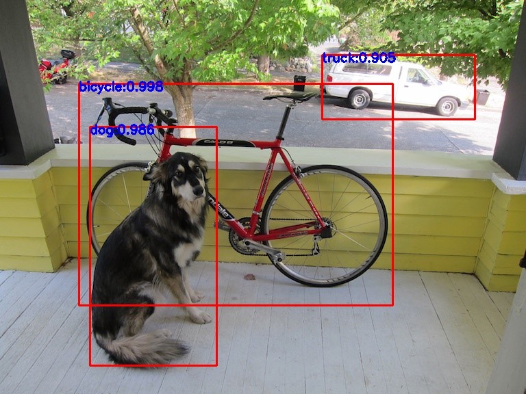
推理前后比较如下:
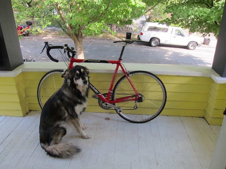
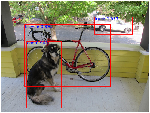
执行在线融合推理,只需要修改代码中的caffe.set_mode_mlu()为caffe.set_mode_mfus()。
执行方式不变,示例如下:python detect.py yolov3_int8.prototxt yolov3.caffemodel
推理前后比较如下前后比较如下:
关键代码:
caffe.set_mode_mfus() # 融合模式
#caffe.set_mode_mlu() # 逐层模式
caffe.set_core_number(1)
caffe.set_batch_size(batch_size)
caffe.set_simple_flag(1)
caffe.set_rt_core("MLU270")
# 加载网络
net = caffe.Net(prototxt, caffemodel, caffe.TEST)
input_name = net.blobs.keys()[0]
# 获取所有标签
label_path = './label_map_coco.txt' # 存储标签的文件
classes = load_classes(label_path) # load_classes函数将所有标签提取出来
# 读取图片做预处理
image_path = './images/image.jpg'
img=cv2.imread(image_path)
img = img[:, :, (2, 1, 0)]
h, w, _ = img.shape
scale = 416/h if w < h else 416/w
# get new w and h
new_w = int(w * scale)
new_h = int(h * scale)
img = cv2.resize(img, (new_w, new_h), interpolation = cv2.INTER_LINEAR)
dim_diff = np.abs(new_h - new_w)
# Upper (left) and lower (right) padding
pad1, pad2 = dim_diff // 2, dim_diff - dim_diff // 2
# Determine padding
pad = ((pad1, pad2), (0, 0), (0, 0)) if h <= w else ((0, 0), (pad1, pad2), (0, 0))
input_img = np.pad(img, pad, 'constant', constant_values=128)
image = np.transpose(input_img, (2, 0, 1))
image=image[np.newaxis, :].astype(np.float32)
images = np.repeat(image, batch_size, axis=0)
# 推理
net.blobs[input_name].data[...]=images
output = net.forward()
# 后处理
output_keys=output.keys()
output=output[output_keys[0]].astype(np.float32)
# 获取(x1, y1, x2, y2, object_conf, class_score, class_pred)
outputs = get_boxes(output, batch_size, img_size=416)
# 对原图画框,标出类别和置信度
out_img = np.array(Image.open(image_path))
for si, pred in enumerate(outputs):
plt.figure()
五、离线推理
1. 生成离线模型:默认在当前目录生成cambricon和offline.cambricon_twins文件
./caffe genoff -model ../quantize/yolov3_int8.prototxt -weights ../quantize/yolov3.caffemodel -mcore MLU270
2. 离线推理:对一张图片进行离线推理,画出目标框和置信度。待推理图片放置在yolov3_pytorch_demo/offline/yolov3_offline_simple_demo/data目录下,离线模型放置在model目录下,执行make.sh在src目录下生成可执行文件,执行run.sh对一张图片进行推理,在result目录下生成推理后的图片。
推理前后比较如下: